This post summarize things I've learned / reviewed over the 1st week of my Quantum Computing Ultralearning challenge. There are two parts: maths (the current one) and articles.
Below math concepts may sound familiar since you might already learn them in your high school or university. But to understand the subsequent weeks' materials wholly, since quantum computing is built on complex number, linear algebra, probability, and other things, a review of fundamental maths knowledge is necessary. Note that the topics listed below are necessary from a newcomer's perspective, but might not sufficient to cover the whole course. Therefore I will also add more stuff to the post over my learning journey so this could become a reference for future readers.
Disclaim: I'm a fan of Gilbert Strang and 3Blue1Brown because of their enthusiastic energy on the topic, as well as an interactive teaching method, thus I mostly used their materials for learning. Actually, when the COVID-19 happened in the US, and the lockdown came, everyone stays at home, I spent every lunchtime, over 2 months, to watch videos of Gilbert Strang's MIT Linear Algebra course to enlight myself (will write about it later ☺).
Complex Numbers #
Material #
Core concepts #
A complex number \(z\) is defined as:
\[ z = x + yi \]
- \( x, y \in \mathbb{R} \)
- \(i\) is an imaginary number, defined as \( i^2 = -1 \)
- \(x\) is the real part of \(z\), notion: \(\Re(z)\)
- \(y\) is the imaginary part of \(z\), notion: \(\Im(z)\)
We can represent complex numbers in the polar complex plane using two numbers \(r\) and \(\varphi\) as defined below:
- Modulus (or magnitude or absolute value) of \(z\) is defined as \(|z| = r = \sqrt{x^2 + y^2}\)
phase (\( \varphi \)) of \(z\) is the angle between the positive real axis (Ox) and the vector Oz.

(image source: Wikipedia)- \( \varphi = artan2(y, x) \). See artan2.
- \( z = r(cos(\varphi) + isin(\varphi)) \)
- \( z = re^{i\varphi} \) (derived from the Euler's formula in the next section).
The complex numbers can help you rotate your vectors easily, just by multiplying!
\[ iz = i(x + yi) = xi + yi^2 = -y + xi = (-y, x) \]
thus multiplying your vector \( (x, y) \) with \( i \) will rotate it 90 degrees counter-clockwise.
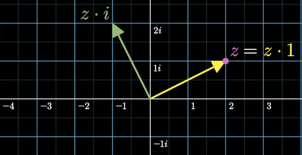
(image source: 24:15 Complex number fundamentals)
\[ e^{ix} = cos(x) + isin(x) \]
When \( x = \pi \), this turns out to be the Euler's identity, one of the most beautiful, yet a simple equation, which connects five important numbers:
\[ e^{i\pi} + 1 = 0 \]
Given a complex number \( z = x \textcolor{green}{+} yi \), the complex conjugate of z is:
\[ z^{*} = \overline{z} = x \textcolor{red}{-} yi \]
In polar form, if \( z = re^{i\varphi} \), then:
\[ z^{*} = \overline{z} = re^{\textcolor{red}{-}i\varphi} \]
Properties:
- \( z\overline{z} = x^2 + y^2 = r^2 \text{ (real number)} \)
- \( \overline{\overline{z}} = z \)
- \( \overline{z+w} = \overline{z} + \overline{w} \)
- \( \overline{z-w} = \overline{z} - \overline{w} \)
- \( \overline{zw} = \overline{z} \text{ } \overline{w} \)
- \( \overline{(\frac{z}{w})} = \frac{\overline{z}}{\overline{w}} \text{ if } w \neq 0 \)
- \( \overline{z^n} = (\overline{z})^n \text{ , } \forall n \in \mathbb{Z} \)
- \( e^{\overline{z}} = \overline{e^z} \)
- \( \log{(\overline{z})} = \overline{\log{(z)}} \text{ if } z \neq 0 \)
Linear Algebra #
Materials #
Important concepts #
(enough to understand quantum computing, since there's a lot more about linear algebra)
Vector, matrix and matrix multiplication:
\[\text{matrix } M =
\begin{bmatrix}
a & b \\
c & d
\end{bmatrix}
\text{ , vector } v =
\begin{bmatrix}
e \\
f
\end{bmatrix}
\]
\[ Mv =
\begin{bmatrix}
ae + bf \\
ce + df
\end{bmatrix}
\]
Transpose: flipping over the main diagonal (from top left to bottom right):
\[M^\intercal =
\begin{bmatrix}
a & c \\
b & d
\end{bmatrix}
\]
Inverse a matrix (more details in the link):
\[M^{-1}M = MM^{-1} = I_2 =
\begin{bmatrix}
1 & 0 \\
0 & 1
\end{bmatrix}
\]
\[ (M^{-1})^{\intercal} = (M^\intercal)^{-1} \]
Vector space: a set of vectors that can be added together or multiplied (scaled) by numbers.
Linear independent: a set of vectors is linearly independent if you cannot create any single one of them using only the linear combinations of the other ones.
Span (linear hull): the smallest vector space that contains a given vector set \(W\), i.e. the set of all the linear combinations of \(W\). If \(\text{span}(W) = S\), we also say \(W \text{ spans } S\), or \(W\) is a spanning set of \(S\).
Basis: a basis of a vector space \(X\) is a linearly independent subset of \(X\) that spans \(X\) ==> smallest possible spanning set of \(X\).
Eigenvalues and Eigenvectors: \(v\) is an eigenvector of \(M\) if there exists some scalar \(\lambda\) (eigenvalue) such that:
\[ Mv = \lambda v \]
Eigenvalues and Eigenvectors are important because with this we can:
- multiplying a vector with a scalar instead of a matrix.
- multiplying a matrix with an eigenvector of it does NOT rotate the eigenvector, only scales it.
Given a matrix \( A \) with complex entries, we can construct the conjugate transpose (or Hermitian transpose, adjoint matrix, or transjugate) of A by following below steps:
- Transpose A. The result is \( A^\intercal \).
- Conjugate every entry of \( A^\intercal \).
Definition:
\[ (A^H)_{ij} = \overline{ A_{ji} } \]
or:
\[ A^{\dagger} = A^* = A^H = (\overline{A})^T = \overline{ A^\intercal } \]
where \( A^{\dagger} \) (pronounced as A dagger) is commonly used in quantum mechanics.
A complex square matrix \( U \) is unitary if its conjugate transpose \( U^{\dagger} \) is also its inverse:
\[ U^{\dagger} U = U U^{\dagger} = I \]
This concept is important because people use it to represent the quantum gates.
The other name: bra–ket notation. The complete definition involves some knowledge out of the scope of this post, so I recommend you read the link above to grasp this concept.
We can (roughly) understand that:
- a bra is a row vector: \(\bra{A} =
\begin{bmatrix}
a & b \\
\end{bmatrix}
\) - a ket is a column vector: \(\ket{B} =
\begin{bmatrix}
c \\
d
\end{bmatrix}
\)
Properties (by definition):
- \( \bra{A}^{\dagger} = \ket{A} \)
- \( \ket{A}^{\dagger} = \bra{A} \)
We also define:
Probability #
(some basic concepts, there's a lot more!)
Random variable: given a random phenomenon, a random variable is a function \( X: \Omega -> \mathbb{E} \), which maps from a set of possible outcomes to a measurable space. For example: in the coin tossing experiment, we can map (the result) head to 0 and tail to 1.
Probability density function (PDF): in the previous example, the random variable is discrete (finite and countable), so you can map each outcome to a number, one by one. But what if the outcome set is continuous? That why you need a probability density function to do the mapping.
Probability: given events \(A_1, A_2, ... A_n \in \Omega \) and \( P(X) \) is the probabilty that \(X\) happens, below properties must be satisfied:
\[ 0 <= P(A_i) <= 1 \]
\[ \sum_{i=1}^{n} P(A_i) = 1 \]
Summary #
But why do we need to know all these mathematical things?
You might ask. Well, since quantum computing is based on quantum mechanics, which is mathematically formulated in Hilbert space, which in turn uses the complex number. A qubit (quantum bit) is not just a single real number like in classical computing, but rather a vector of two complex numbers, and in order to apply operations on it, you will need the quantum gates, which can be seen as matrices, time for linear algebra! Finally, the value of a qubit is not deterministic but varies between 0 and 1, thus you need probability to represent it.
I will explain the alien topics above in the upcoming posts of my quantum challenge.
Is there a no-math road toward quantum wisdom?
Sadly, no, at least until this moment.
Since you've made it this far, sharing this article on your favorite social media network would be highly appreciated!
For feedback, ping me on Twitter.
All the information on this blog are my own opinions and do NOT represent the views or opinions of any of my past or current employers.
Published