"You can't use an old map to explore a new world."
Albert Einstein
This post summarizes things I've learned/reviewed over the 2nd week of my Quantum Computing Ultralearning challenge, and it also tries to outline a map of knowledge of the Quantum Computing field, so future readers will know how to start studying as well as where they might end up landing.
We will begin with some background review on complexity theory and how to distinguish Quantum Information vs Quantum Computing. After that is basic knowledge on Qubit and Quantum Gates & Circuit. Then we'll discover the power of superposition, destructive interference, and entanglement in solving hard computational problems. Near the end are the limitations and real-life applications of this field. Finally, there's s fun section.
Note that there is a lot of detailed knowledge from [1], but this post does not contain them since it will be more suitable to explain them in their corresponding weeks of the challenge.
Background on Complexity #
If you don't have a computer science background, I recommend you reading more about the computational complexity theory to have a deeper understanding of the below notations. Here is a brief summary:
- NP (nondeterministic polynomial time): the class of problems for which you can check if a solution is correct or not in polynomial time.
- P (polynomial time): the class of problems for which you can find solutions (and of course check if one solution is correct) in polynomial time. P is contained within NP.
- NP-complete problems: the hardest of the NP problems. But if you can find an efficient algorithm to solve any of them, then you can solve all the other NP problems in polynomial time.
Also: P versus NP problem and NP-hard.
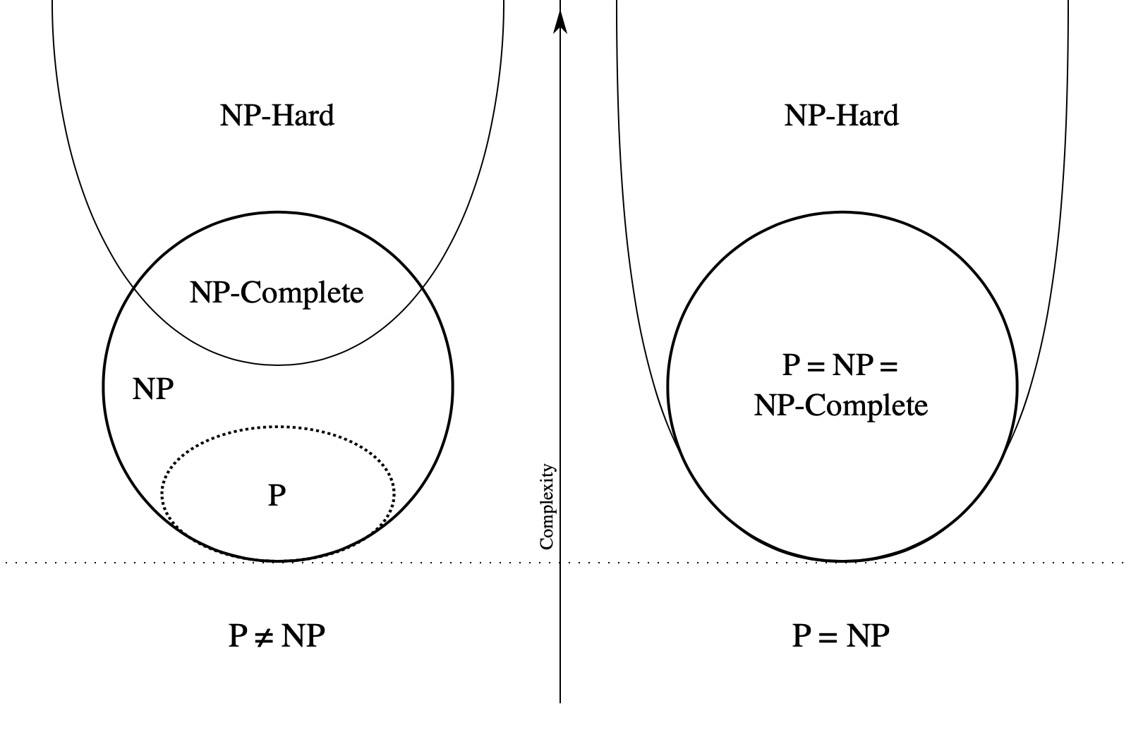
image source
One of the first thing newcomers should know is how to distinguish these two terms:
Quantum Information is
"the information of the state of a quantum system. It is the basic entity of study in quantum information theory, and can be manipulated using quantum information processing techniques." [3]
"Its main focus is in extracting information from matter at the microscopic scale." [3]
and Quantum Computing is
"the use of quantum phenomena such as superposition and entanglement to perform computation. The study of quantum computing is a subfield of quantum information science." [4]
Quantum Information is more about theoretical concepts and physics, while Quantum Computing is one of its applications, which focuses on making computation more efficient. My interest is the latter aspect, not only because Quantum Computing is the name of this ultralearning, but also that is what I would like to work on: speeding up computational processes using quantum weirdness.
Qubit #
What is a qubit?
According to Prof. Scott Aaronson at the University of Texas at Austin:
"A qubit may be a particle such as an electron, with "spin up" representing 1, "spin down" representing 0, and quantum states called super-positions that involve spin up and spin down simultaneously." [2]
The image below demonstrates states of a qubit: 0 and 1 are similar to the values of a classical bit, but a qubit also has other states, which lie "somewhere between" 0 and 1.
We call these new states the superposition: not entire 0 neither entire 1 but both of them at the same time!
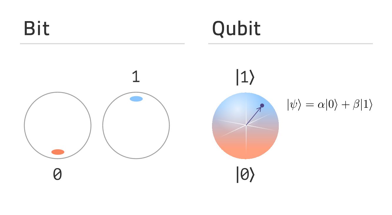
image source: SINTEFblog.
\(\ket{0}\), \(\ket{1}\) and \(\ket{\psi}\) are diarc notation, which has the same meaning as column vectors:
\[\ket{0} =
\begin{bmatrix}
1 \\
0
\end{bmatrix}
\qquad\qquad
\ket{1} =
\begin{bmatrix}
0 \\
1
\end{bmatrix}
\]
By definition, \(\ket{\psi}\) is a linear combination of \(\ket{0}\) and \(\ket{1}\) :
\[\ket{\psi} =
\begin{bmatrix}
\alpha \\
\beta
\end{bmatrix}
\]
where \(\alpha\) and \(\beta\) are complex numbers. In this case, they are the probability amplitudes of the qubit \(\ket{\psi}\), so that when we measure it, the probability of outcome \(\ket{0}\) is \(|\alpha|^2\) and probability of outcome \(\ket{1}\) is \(|\beta|^2\). \(\alpha\) and \(\beta\) are also constrained by the equation below:
\[ |\alpha|^2 + |\beta|^2 = 1 \]
IMPORTANT: when you measure a qubit, it will collapse to a basis state (either \(\ket{0}\) or \(\ket{1}\) in this case). Why? Because observing a qubit changes its state. This also means information will be lost when you try to read your qubit's value.
Quantum Gates and Circuit #
To perform operations on a qubit, we will need to use the quantum gates. Notice that each gate operator is represented as a matrix instead of a logical operator (AND, OR, NOT, XOR, etc.) as in classical logic gates. This difference comes from the way we see a qubit: as a vector instead of a scalar.
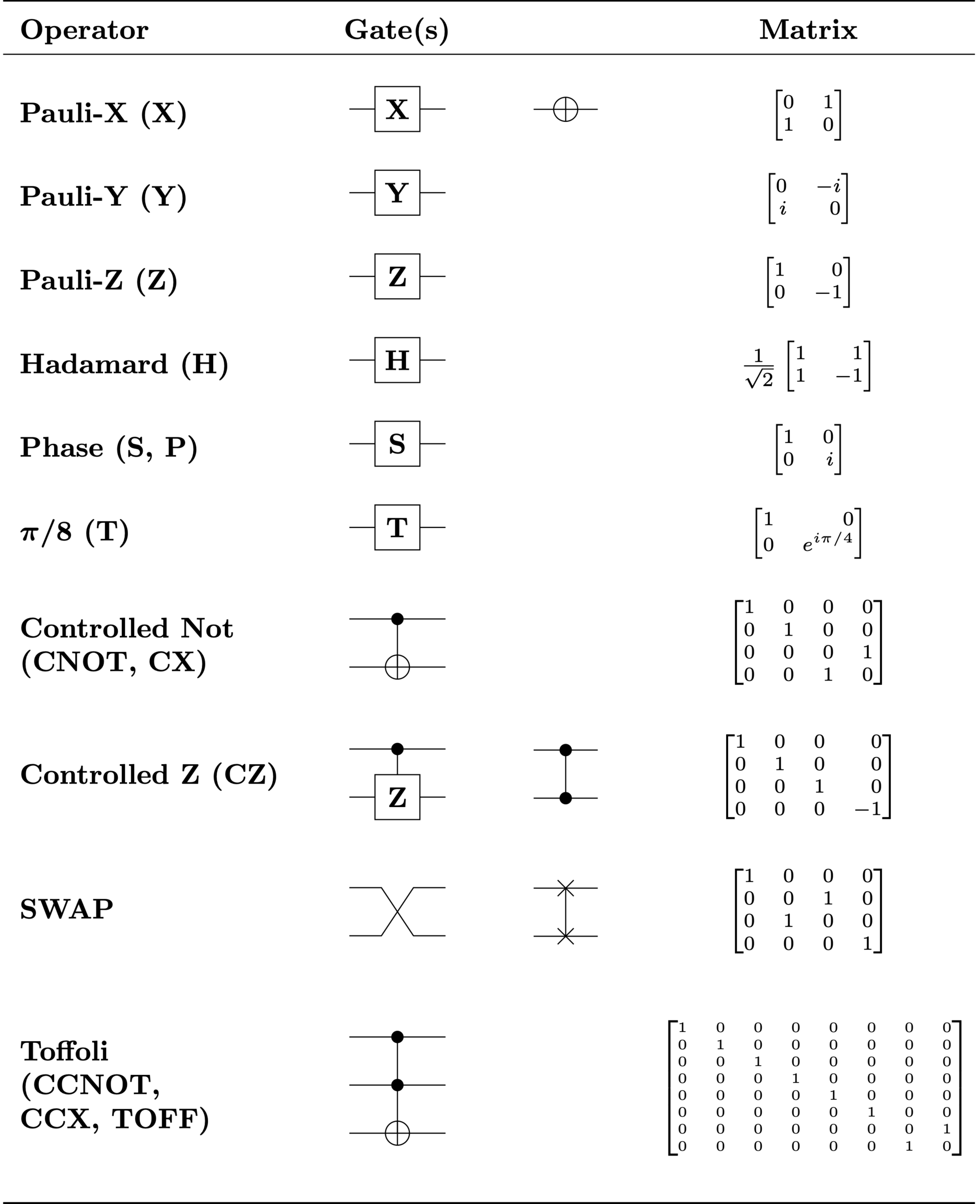
Some common quantum gates from image source.
Similar to classical computing, to leverage the power of multiple qubit systems, we need to have quantum circuits:
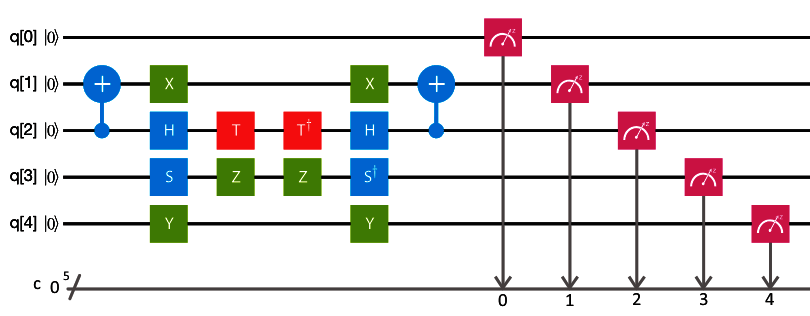
image source
This section is just an overview, we will consider qubit, quantum gates, and quantum circuit thoroughly in week 5, on their mathematical properties together with some programming exercises.
Until now, we have only talked about the definitions of quantum computing fundamental elements, but how do they help us build a computational model that is stronger than the classical one? See an answer below:
"Imagine that we have \(1000\) particles and that each particle, when measured, can be found to be either spinning up or spinning down. To describe the quantum state of this collection of particles, one must specify a number for every possible result of measuring the particles.
For example, an amplitude is needed for the possibility that all \(1000\) particles will be found spinning up, another amplitude for the possibility of finding that the first \(500\) particles are spinning up and that the remaining \(500\) are spinning down, and so on. There are \(2^{1000}\) possible outcomes, or about \(10^{300}\), so that is how many numbers are needed - more than there are atoms in the visible universe! The technical terminology for this situation is that the \(1000\) particles are in a superposition of those \(10^{300}\) states." [2]
Wow, so powerful! Does that mean we can solve all NP problems in polynomial-time using quantum computers?
Not quite yet... Despite the capacity of \(2^n\) states with just \(n\) qubits, remember that when we try to measure them, information loss happens. That's why you cannot just implement an exponential classical algorithm on a quantum computer and hope that it will run in polynomial-time.
Does that mean the advantage of superposition is just an illusion?
No, actually, because we have another way to leverage that property, and it requires a new mindset for the problems and algorithms. We will discuss it in the next section.
The link in this section's title contains a lot of maths and some readers might enjoy them, but let's make it easier for us human beings to understand by reading the quotes below:
"We still have tricks we can play to wring some advantage out of the quantum particles. Amplitudes can cancel out when positive ones combine with negative ones, a phenomenon called destructive interference." [2]
"A good quantum computer algorithm ensures that computational paths leading to a wrong answer cancel out and that paths leading to a correct answer reinforce." [2]
Wait, what does that mean?
Here is an illustration: do you know the Galton Board (or bean machine or quincunx)? Below is an image of it:

image source
The rule is simple: you drop balls from the top and they will bounce their way down to the bottom. Since the chances of bouncing to the left or the right when a ball hitting a peg are equal (50/50), so the final number of balls should be approximately equal in every column, right?
Wrong! The interesting thing is that it forms a bell-shaped curve, or in mathematical terms: a normal distribution.
We can roughly understand the way a good quantum computer algorithm works is similar to the Galton Board: the "correct paths" (center columns) are reinforced while the "wrong paths" (peripheral columns) are canceled out.
That sounds magical. Is it really possible? Yes:
"In 1994 Peter Shor showed how a quantum computer could factor an n-digit number using a number of steps that increases only as about \(n^2\) — in other words, in polynomial-time. As mentioned earlier, the best algorithm known for classical computers uses a number of steps that increases exponentially" [2]
Wonderful! But can we do it with ALL \(NP\) problems?
Sadly, we don't know if we can (or cannot) do that yet. More details in the limitations section.
From the link in the section's title:
"Quantum entanglement is a physical phenomenon that occurs when a pair or group of particles is generated, interact, or share spatial proximity in a way such that the quantum state of each particle of the pair or group cannot be described independently of the state of the others, including when the particles are separated by a large distance."
In other words, after you bound two qubits together, no matter how far they are from each other, there will still have some kind of connection between them.

Source: Scientists Just Unveiled The First-Ever Photo of Quantum Entanglement
This property enables the ability to transfer information in long-distance using quantum mechanics, and based on that, we can build the quantum internet.
Wait, does that mean you could send information faster than the speed of light?
The short answer is no, the long answer is in the limitations section.
We will also deep dive into this topic in week 8 of the challenge.
Limitations #
First let's talk about the limitations of quantum information, in other words, the constraints of reality governed by the laws of physics. From [3]:
So what are the abilities of a quantum computer?
Maybe we can answer that question by substituting an easier one: what a quantum computer cannot do?
It CANNOT transfer information faster than light by using quantum entanglement. Because the process requires transferring additional classical information (which is, by using non-quantum technologies, aren't faster than light) [1].
It CANNOT compress \(2^n\) bits using \(n\) qubit. Because information loss happens when you measure a qubit. But there is some interesting idea such as the superdense coding, which we will discover in week 8.
Can it solve all the NP problems? We don't know yet:
To create his algorithm, Shor exploited certain mathematical properties of composite numbers and their factors that are particularly well suited to producing the kind of constructive and destructive interference that a quantum computer can thrive on. The NP-complete problems do not seem to share those special properties. To this day, researchers have found only a few other quantum algorithms that appear to provide a speedup from exponential to polynomial-time for a problem. [2]
Is there an efficient quantum algorithm to solve NP-complete problems? Despite much trying, no such algorithm has been found — though not surprisingly, computer scientists cannot prove that it does not exist. After all, we cannot even prove that there is no polynomial-time classical algorithm to solve NP-complete problems. [2]
What we can say is that a quantum algorithm capable of solving NP-complete problems efficiently would, like Shor’s algorithm, have to exploit the problems’ structure, but in a way that is far beyond present-day techniques. One cannot achieve an exponential speedup by treating the problems as structureless "black boxes", consisting of an exponential number of solution to be tested in parallel. [2]
The "black boxes" approach has another name which is more familiar with computer science student: the Brute-force search, in which you try every possible solution until you find the correct one.
The Grover's algorithm, an important algorithm developed in 1996 by Lov Grover of Bell Laboratories, shows that quantum computer can find the correct solution in just \(\sqrt{S}\) steps instead of \(S\) steps as in classical computing, where \(S\) is the number of possible solutions.
Note that since \(S\) grows exponentially as the problem size increases, \(\sqrt{S}\) does not grow polynomially, but it's still a remarkable speedup.
This is also the best a "black-boxes" algorithm can do:
In 1994 researchers had shown that any black-box quantum algorithm needs at least \(\sqrt{S}\) steps. [2]
So is there anything for us to do?
Yes, we can try to find new efficient quantum algorithms to solve NP-complete problems, but remember:
If such algorithms existed, however, they would have to exploit the problems’ structure in ways that are unlike anything we have seen, in much the same way that efficient classical algorithms for the same problems would have to. Quantum magic by itself is not going to do the job. [2]
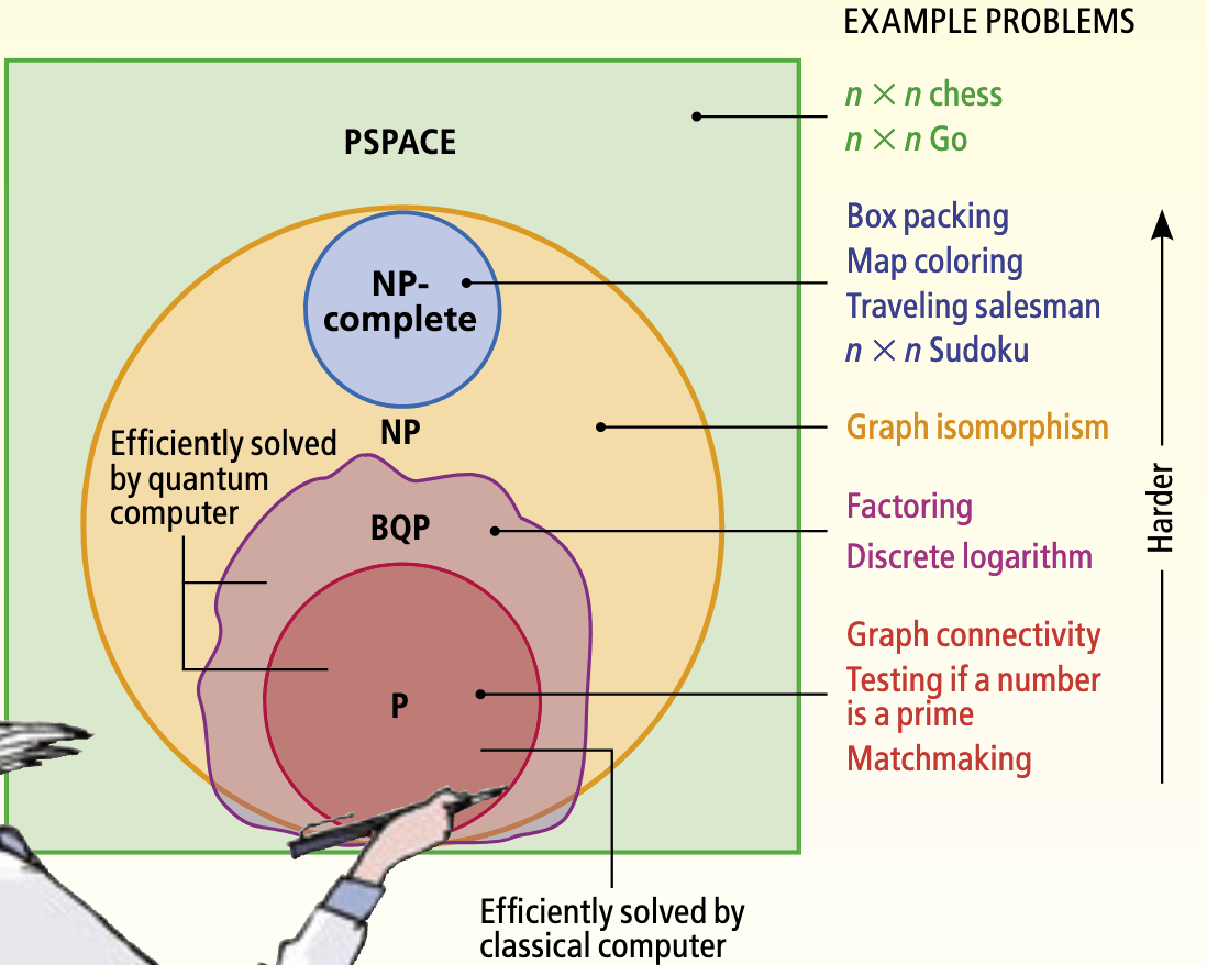
Below is a diagram from [2] to summarize the current abilities of quantum computer and classical computer:
Finally, the more qubits you add to a quantum system, the higher the error rate it has, which prevents us from achieving a really efficient quantum computer:
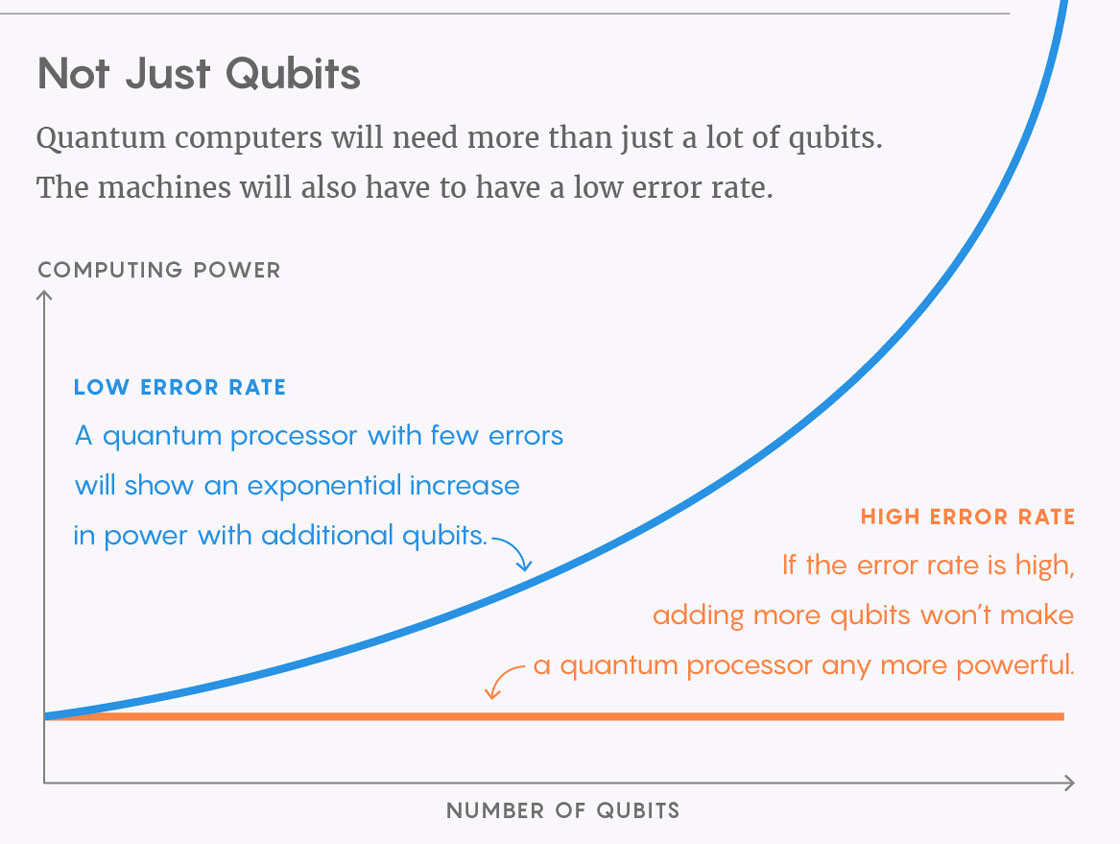
image source
Real-life applications #
Enough of theory, it's time to change the world!
In this section, we go through some real-life applications of quantum information and quantum computing.
Quantum physics simulation:
The killer application of Quantum Computing.
A fundamental problem for chemistry, nanotechnology, and other fields, important enough that Nobel Prizes have been awarded even for partial progress. [2]
Quantum key distribution: a new secure communication method using quantum mechanics.
Fourier transform based quantum algorithms:
- Shor's algorithm: polynomial-time quantum computer algorithm for integer factorization. Note that the current internet security protocol depends on the unsolvable-in-polynomial-time of the integer factorization problem, and a breakthrough in quantum computing could break all these locks of the current system.
- Other algorithms.
Amplitude amplification based algorithms:
Quantum walks based algorithms:
Solving linear systems of equations.
Quantum machine learning: improve computational speed and data storage of machine learning algorithms.
In 2002, Scott Aaronson proved that the collision problem (finding two items that are identical in a long list) cannot be solved efficiently using the black box approach since they need exponential time:
If there were a fast quantum algorithm to solve this problem, many of the basic building blocks of secure electronic commerce would be useless in a world with quantum computers. [2]
Fun #
Schrödinger's Pants:
Pants are shorter than the wearer’s shirt and it appears the wearer has no pants. The wearer is simultaneously both wearing and not wearing pants. Much like Schrödinger’s cat; which is simultaneously dead and alive in an unopened box. Source.

image source
Further readings #
- The complexity of theorem-proving procedures - by Stephen A. Cook of the University of Toronto.
- BQP: Bounded-Error Quantum Polynomial-Time
- NP-Complete Problems and Physical Reality - Scott Aaronson
- Quantum Computer Science: An Introduction - N. David Mermin.
- Shor, I’ll Do It - Scott Aaronson
- Quantum Computing since Democritus - Lecture notes by Scott Aaronson
References #
1. Book: Chapter 1 of Quantum Computation and Quantum Information (10th Anniversary Edition).
2. The Limits of Quantum Computers - Scott Aaronson.
3. Quantum Information - Wikipedia.
4. Quantum Computing - Wikipedia.
5. What Quantum Computing Isn't - Scott Aaronson.
6. We’re Close to a Universal Quantum Computer, Here’s Where We're At.
Since you've made it this far, sharing this article on your favorite social media network would be highly appreciated!
For feedback, ping me on Twitter.
All the information on this blog are my own opinions and do NOT represent the views or opinions of any of my past or current employers.
Published