Quantum Computing Ultralearning - Week 3 & 4: Quantum Mechanics

"I think I can safely say that nobody understands quantum mechanics." - Richard Feynman

This post summarizes things I've learned/reviewed over the 3rd and 4th week of my Quantum Computing Ultralearning challenge, and should be considered as study notes instead of a fully-explained-and-very-detailed article on quantum mechanics, since this topic is complex and other experts have done that work before (see references).

We will start from an overview of quantum mechanics, then consider the four postulates: states, dynamics, measurement, and composite system. The final parts are the summary and further readings.

What is Quantum Mechanics #

It is NOT a fully specified physical theory.
It is a framework, which can be used to construct physical theories.
Analogy: quantum mechanics ~ operating system, while physical theories ~ softwares.

"It's a set of four postulates that provide a mathematical framework for describing the universe and everything in it." [2]

Postulate 1 - States #

"Associated to any physical system is a complex vector space known as the state space of the system. If the system is isolated, then the system is completely described by its state vector, which is a unit vector in the system's state space." [2]

Every physical system has a state space: qubits, humans, the universe, etc.
The 1st postulate does NOT tell us how to find the state space of every physical system, we'll need to figure it out case by case.
How about non-isolated physical systems?
--> They do NOT have their own quantum state!
For example: with two entangled qubits below, you cannot assign a quantum state to only one of them.
\[ \frac{\ket{00} + \ket{11}}{\sqrt{2}} \]

Postulate 2 - Dynamics #

"The evolution of an isolated quantum system is described by a unitary matrix acting on the state space of the system. That is, the state \( \ket{\psi} \) of the system at a time \( t_1 \) is related to the state \( \ket{\psi'} \) at a later time \( t_2 \) by a unitary matrix, \( U: \ket{\psi'} = U\ket{\psi} \). That matrix \( U \) may depend on the times \( t_1 \) and \( t_2 \), but does not depend on the states \( \ket{\psi} \) and \( \ket{\psi'} \)." [2]

This means the dynamics of a quantum system through time.
Why do we need unitary matrices? Why not just some general matrices?
--> One of the reasons: unitary matrices are the only matrices that preserve length --> quantum states remain normalized --> when you measure them, the probabilities of outcomes sum to one.
Note that the above 2nd postulate talks about discrete (non-continuous) time.
With continuous time, we have the Schrodinger equation:
\[ i\frac{d\ket{\psi}}{dt} = H\ket{\psi} \]
where \( H \) is a (fixed) hermitian matrix known as the Hamiltonian of the system.

We can get the equation to relate the discrete-time states at \(t_1\) and \(t_2\) by solving the Schrodinger equation, which gives:
\[ \ket{\psi_{t2}} = e^{-iH(t_2-t_1)}\ket{\psi_{t_1}} \]

Postulate 3 - Measurement #

"Quantum measurements are described by a collection \( \{ M_m \} \) of measurement operators. Each \(M_m\) is a matrix acting on the state space of the system being measured. The index \(m\) takes values corresponding to the measurement outcomes that may occur in the experiment. If the state of the quantum system is \(\ket{\psi}\) immediately before the measurement then the probability that result \(m\) occurs is given
\[ p(m) = \bra{\psi} M_m^{\dagger} M_m \ket{\psi} \space , \]
and the state of the system after the measurement, often called the posterior state, is
\[ \frac{ M_m\ket{\psi }}{ \sqrt{ \bra{\psi} M_m^{\dagger} M_m \ket{\psi} } } \]
It's worth noting that:
(a) the denominator is just the square root of the probability \(p(m)\).
(b) this is a properly normalized quantum state.

The measurement operators satisfy the completeness relation:
\[ \sum_m{ M_m^{\dagger} M_m = I } \]
" quoted from [2].

The idea is that the outcomes of quantum measurements are NOT deterministic but rather following a probabilistic distribution.
This is somewhat counter-intuitive, but we have an intuitive explanation in [3].
How to prove it? [3] also summarizes an approach using the Clauser-Horne-Shimony-Holt (CHSH) inequality.

Postulate 4 - Composite System #

"The state space of a composite physical system is the tensor product of the state spaces of the component physical systems.
Moreover, if we have systems numbered \(1\) through \(n\), and system number \(j\) is prepared in the state \(\ket{\psi_j}\), then the joint state of the total system is just the tensor product of the individual states:
\[\ket{\psi_1} \otimes \ket{\psi_2} \otimes \space ... \otimes \space \ket{\psi_n}\]" quoted from [2].

What is a composite physical system? --> Example: a multi-qubits system:
\[ \frac{\ket{00} + \ket{11}}{\sqrt{2}} \]
On notation: \( \ket{00} = \ket{0} \ket{0} = \ket{0} \otimes \ket{0} \) .

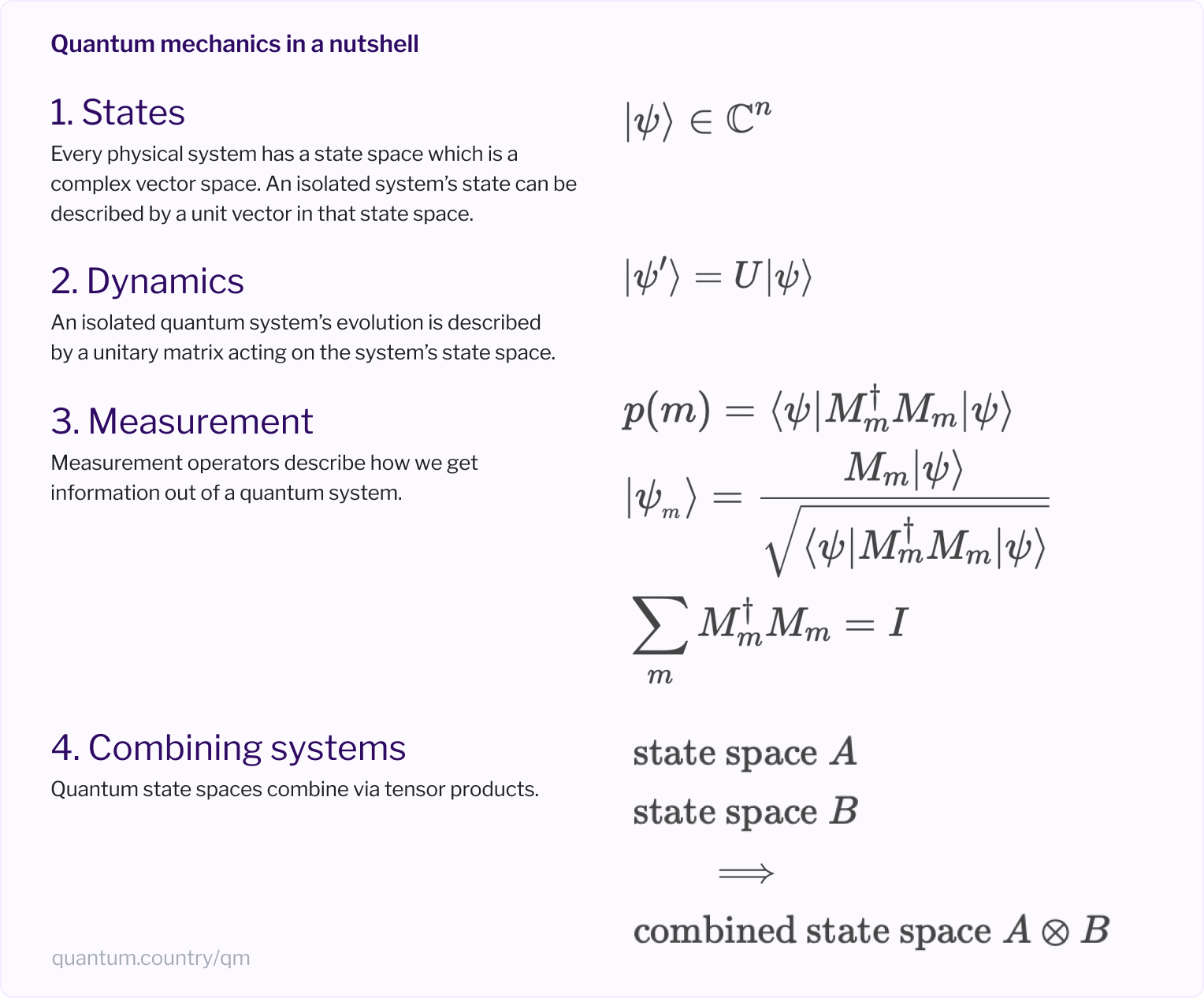
Summary #

Finally, to recap the main points of this post, we thankfully have the below image, which is from the section Quantum mechanics in a nutshell of [2]:

One thing I should have done better: studying this topic after already grasped the qubit and quantum circuits ones, since there are a lot of examples to illustrate the above concepts using quantum circuits. This is also the recommended order in [2].

References #

1. Book: Chapter 2 of Quantum Computation and Quantum Information (10th Anniversary Edition).
2. Quantum mechanics distilled - Andy Matuschak and Michael Nielsen.
3. Why the world needs quantum mechanics - Michael Nielsen.
4. The postulates of quantum mechanics I: states and state space - Michael Nielsen.
5. The postulates of quantum mechanics II: dynamics - Michael Nielsen.
6. The postulates of quantum mechanics III: measurement - Michael Nielsen.

Since you've made it this far, sharing this article on your favorite social media network would be highly appreciated!
For feedback, ping me on Twitter.

All the information on this blog are my own opinions and do NOT represent the views or opinions of any of my past or current employers.

Published 19 Jan 2021