This post summarizes things I've learned over the 5th week of my Quantum Computing Ultralearning challenge, and should be considered as study notes instead of a fully-explained-and-very-detailed article on quantum bits (qubits), since this topic is complex and other experts have done that work before (see references).
Qubit #
Qubit, like the classical bit, is an abstract mathematical object. [2]
But in order to build quantum computers, people need to realize them in physical systems. To store a qubit, we can use an electron, a photon, an atom, or other methods as in the "Physical implementations" section of [1].
Similar to a classical bit, a qubit also has a state, which is also an abstract mathematical object [2].
But unlike a scalar value (0 or 1) of a bit's state, the state of a qubit is a 2-dimensional vector of complex numbers:
\[ \ket{\psi} = \begin{bmatrix} \alpha \\ \beta \end{bmatrix} \]
where \(\alpha\) and \(\beta\) are the amplitudes of states \(0\) and \(1\), respectively, which hold the normalization constraint:
\[ |\alpha|^2 + |\beta|^2 = 1 \]
The notation \(\ket{\psi}\) is called the Ket of \(\psi\), we also use the Bra of \(\psi\), which is written as \(\bra{\psi}\), and is defined as:
\[ \bra{\psi} = \begin{bmatrix} \alpha^* & \beta^* \end{bmatrix} \]
where \( \alpha^* \) is the complex conjugate of \(\alpha\).
The above vector is called the state vector of the qubit, and the vector space of all these state vectors is the state space.
You might ask: Why two-dimensional vector? Why complex numbers? What do they mean, physically?
See this:
"These are good questions. But they do take some time to answer. For context consider that the discovery of quantum mechanics wasn’t a single event, but occurred over 25 years of work, from 1900 to 1925. Many Nobel prizes were won for milestones along the way. That includes Albert Einstein’s Nobel Prize, won primarily for work related to quantum mechanics (not relativity, as people sometimes assume).
When some of the brightest people in the world struggle for 25 years to develop a theory, it’s not an obvious theory! In fact, the idea of describing a simple quantum system using a complex vector in two dimensions summarizes much of what was learned over that 25 years. In that sense, it’s quite a simple and beautiful statement. But it’s not an obvious statement, and it’s not unreasonable that it might take a few hours to understand. That’s better than taking 25 years to understand!" [2]
Important states #
So important, that they have their own notations:
| Ket | Bra |
|---|
| \( \ket{0} = \begin{bmatrix} 1 \\ 0 \end{bmatrix} \) | \( \bra{0} = \begin{bmatrix} 1 & 0 \end{bmatrix} \) |
| \( \ket{1} = \begin{bmatrix} 0 \\ 1 \end{bmatrix} \) | \( \bra{0} = \begin{bmatrix} 0 & 1 \end{bmatrix} \) |
| \( \ket{+} = \begin{bmatrix} \frac{1}{\sqrt{2}} \\ \frac{1}{\sqrt{2}} \end{bmatrix} = \frac{ \ket{0} + \ket{1} }{\sqrt{2}} \) | \( \bra{+} = \begin{bmatrix} \frac{1}{\sqrt{2}} & \frac{1}{\sqrt{2}} \end{bmatrix} = \frac{ \bra{0} + \bra{1} }{\sqrt{2}} \) |
| \( \ket{-} = \begin{bmatrix} \frac{1}{\sqrt{2}} \\ \frac{-1}{\sqrt{2}} \end{bmatrix} = \frac{ \ket{0} - \ket{1} }{\sqrt{2}} \) | \( \bra{-} = \begin{bmatrix} \frac{1}{\sqrt{2}} & \frac{-1}{\sqrt{2}} \end{bmatrix} = \frac{ \bra{0} - \bra{1} }{\sqrt{2}} \) |
| \( \ket{i} = \begin{bmatrix} \frac{1}{\sqrt{2}} \\ \frac{i}{\sqrt{2}} \end{bmatrix} = \frac{ \ket{0} + i\ket{1} }{\sqrt{2}} \) | \( \bra{i} = \begin{bmatrix} \frac{1}{\sqrt{2}} & \frac{-i}{\sqrt{2}} \end{bmatrix} = \frac{ \bra{0} - i\bra{1} }{\sqrt{2}} \) |
| \( \ket{-i} = \begin{bmatrix} \frac{1}{\sqrt{2}} \\ \frac{-i}{\sqrt{2}} \end{bmatrix} = \frac{ \ket{0} - i\ket{1} }{\sqrt{2}} \) | \( \bra{-i} = \begin{bmatrix} \frac{1}{\sqrt{2}} & \frac{i}{\sqrt{2}} \end{bmatrix} = \frac{ \bra{0} + i\bra{1} }{\sqrt{2}} \) |
We can also write the state of \(\ket{\psi}\) and \(\bra{\psi}\) as:
\[ \ket{\psi} = \alpha\ket{0} + \beta\ket{1} \]
\[ \bra{\psi} = \alpha^* \bra{0} + \beta^* \bra{1} \]
Note that \( \ket{0} \) is NOT 0, since \( \ket{0} = \begin{bmatrix} 1 \\ 0 \end{bmatrix} \), while \( 0 = \begin{bmatrix} 0 \\ 0 \end{bmatrix} \).
Why are these states special? See the next section.
Orthonormal bases #
We call a set of linear independent vectors an orthonormal basis if:
- All of them are normalized. For example: \( \braket{0|0} = 1 \) .
- They are orthogonal to each other. For example: \( \braket{0|1} = 0 \) .
The previous section's states are important because some pairs of them satisfy the mentioned conditions, i.e. each of the below pairs form an orthonormal basis:
- \(\ket{0}\) and \(\ket{1}\) form a computational basis (or canonical basis).
- \(\ket{+}\) and \(\ket{-}\) form a Hadamard basis.
- \(\ket{i}\) and \(\ket{-i}\) .
Why do we care about this? See the Measurement section.
Superposition #
When a qubit is NOT in the states \(\ket{0}\) or \(\ket{1}\), we say it is in a superposition state.
In some previous posts, I wrote that superposition means the qubit is "simultaneously" in both \(\ket{0}\) and \(\ket{1}\), but this explanation seems inaccurate, according to Michael Nielsen:
"I must confess, I don't understand what people mean by this. As far as I can tell, what they're trying to do is explain the quantum state in terms of classical concepts they're already familiar with. But I can't make much sense of it – saying \(0.6\ket{0}+0.8\ket{1}\) is simultaneously in the \(\ket{0}\) state and the \(\ket{1}\) state seems like word salad." [2]
Then how should we understand this concept?
Currently, there's no other explanation, maybe I will able to find out in the future weeks.
"But the trouble is that there is enormous disagreement amongst physicists themselves about how to think about the quantum state. Indeed, many active researchers are trying to understand what the correct way of thinking about the quantum state is, exploring multiple approaches in great depth. So we’re going to defer worrying too much about this until later." [2]
Visualization: the Bloch Sphere #
A way to visualize a qubit state is using the Bloch Sphere:

image source
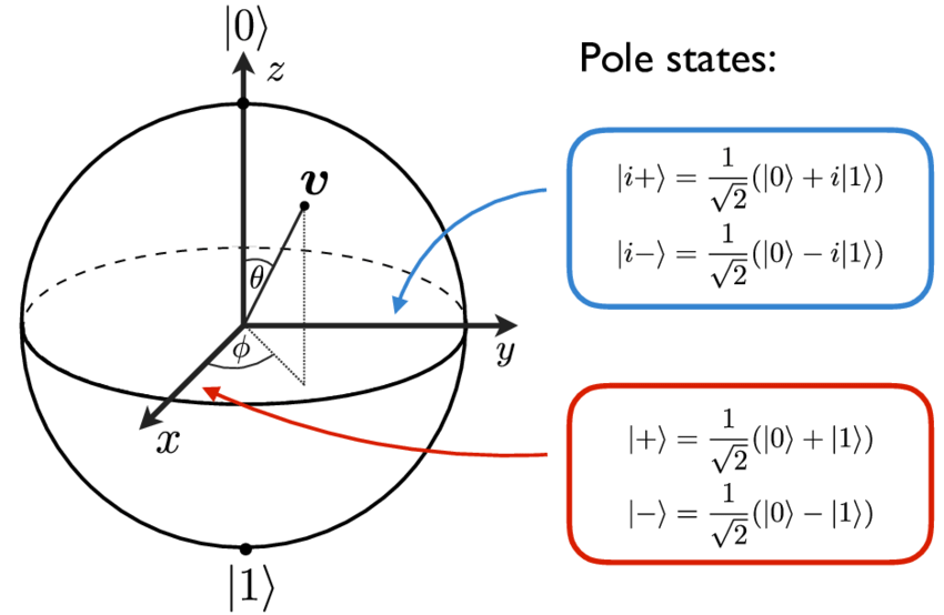
image source
How do we derive the formula \( \ket{\psi} = cos{\frac{\phi}{2}} \ket{0} + e^{i\varphi} sin{\frac{\phi}{2}} \ket{1} \) ?
See [4] for details.
Measurement #
Similar to a classical bit, in order to know the value of a qubit, we need to measure it. But the weird property of quantum mechanics is that: measurement also changes the qubit's state!
Suppose we have a qubit \( \ket{\psi} = \alpha\ket{0} + \beta\ket{1} \),
after being measured in the computational basis \( ( \ket{0} , \ket{1} ) \), it would collapse into:
- \(\ket{0}\) with a probability of \(\alpha^2\),
- or \(\ket{1}\) with a probability of \(\beta^2\).
Note that there are different measurement methods (see [5]), as well as different bases to be used. For example, you could measure the mentioned qubit in the Hadamard basis, and it would collapse into \(\ket{+}\) or \(\ket{-}\) instead of \(\ket{0}\) ot \(\ket{1}\).
Multi-qubit system #
How to represent more than one qubits?
You could represent 2 qubits could in a 4-dimensional linear vector space, spanned by the below basis states:
\[
\ket{00} = \begin{bmatrix} 1 \\ 0 \\ 0 \\ 0 \end{bmatrix} \ \ \text{,} \ \
\ket{01} = \begin{bmatrix} 0 \\ 1 \\ 0 \\ 0 \end{bmatrix} \ \ \text{,} \ \
\ket{10} = \begin{bmatrix} 0 \\ 0 \\ 1 \\ 0 \end{bmatrix} \ \ \text{,} \ \
\ket{11} = \begin{bmatrix} 0 \\ 0 \\ 0 \\ 1 \end{bmatrix}
\]
In general:
\[
\ket{\psi\Phi} = \begin{bmatrix} \alpha \\ \beta \\ \delta \\ \gamma \end{bmatrix}
= \alpha\ket{00} + \beta\ket{01} + \delta\ket{10} + \gamma\ket{11}
\]
Thus \(n\) qubits will need a \(2^n\) dimensional linear vector space.
To develop the intuition for understanding a multi-qubit system, let's go through an example. Consider two qubit states:
\[\ket{+} = \begin{bmatrix} \frac{1}{\sqrt{2}} \\ \frac{1}{\sqrt{2}} \end{bmatrix} = \frac{ \ket{0} + \ket{1} }{\sqrt{2}} \]
\[ \ket{-} = \begin{bmatrix} \frac{1}{\sqrt{2}} \\ \frac{-1}{\sqrt{2}} \end{bmatrix} = \frac{ \ket{0} - \ket{1} }{\sqrt{2}} \]
How do we represent \( \ket{+-} \) and \( \ket{--} \)?
By using tensor product:
\[\ket{+-} = \ket{+} \otimes \ket{-}
= \begin{bmatrix} \frac{1}{\sqrt{2}} \\ \frac{1}{\sqrt{2}} \end{bmatrix}
\otimes \begin{bmatrix} \frac{1}{\sqrt{2}} \\ \frac{-1}{\sqrt{2}} \end{bmatrix}
= \begin{bmatrix} \frac{1}{2} \\ \frac{-1}{2} \\ \frac{1}{2} \\ \frac{-1}{2} \end{bmatrix} \ \ \ (1)
\]
\[\ket{--} = \ket{-} \otimes \ket{-}
= \begin{bmatrix} \frac{1}{\sqrt{2}} \\ \frac{-1}{\sqrt{2}} \end{bmatrix}
\otimes \begin{bmatrix} \frac{1}{\sqrt{2}} \\ \frac{-1}{\sqrt{2}} \end{bmatrix}
= \begin{bmatrix} \frac{1}{2} \\ \frac{-1}{2} \\ \frac{-1}{2} \\ \frac{1}{2} \end{bmatrix}
\]
Now let's think backward: given a state vector, can we determine the states of its component qubit?
In general, we cannot!
For example, to find out the two qubits \( \ket{\psi} = \alpha\ket{0} + \beta\ket{1} \) and \( \ket{\Phi} = \delta\ket{0} + \gamma\ket{1} \) which construct the state vector (1) above, we have:
\[\begin{bmatrix}
\alpha\delta = \frac{1}{2} \\
\alpha\gamma = \frac{-1}{2} \\
\beta\delta = \frac{1}{2} \\
\beta\gamma = \frac{-1}{2} \end{bmatrix}
\]
\( => \alpha = \beta \) because both of them equal to \(\frac{1}{\delta+\gamma}\) ,
and \( \delta = -\gamma \) because \( \delta = \frac{1}{\alpha+\beta} \) and \( \gamma = \frac{-1}{\alpha+\beta} \)
We also have \( \alpha^2 + \beta^2 = 1 \) and \( \delta^2 + \gamma^2 = 1 \), thus there are two solutions:
- \( \alpha = \beta = \frac{1}{\sqrt{2}} \) and \( \delta = \frac{1}{\sqrt{2}} \) and \( \gamma = \frac{-1}{\sqrt{2}} \), or
- \( \alpha = \beta = \frac{-1}{\sqrt{2}} \) and \( \delta = \frac{-1}{\sqrt{2}} \) and \( \gamma = \frac{1}{\sqrt{2}} \)
In other words, for (1), we cannot distinguish its two solutions: \( \ket{+-} \) and \( \frac{ -\ket{0} -\ket{1} }{\sqrt{2}} \frac{ -\ket{0} +\ket{1} }{\sqrt{2}} \).
Programming #
https://colab.research.google.com/drive/1s9ap5V6wns2WIFBM4DKbkDIoD86UMa7B?usp=sharing
References #
1. Qubit - Wikipedia
2. Quantum computing for the very curious - Part I: The state of a qubit - Andy Matuschak and Michael Nielsen.
3. Qubit - microsoft/QuantumKatas
4. Representing Qubit States - Qiskit.org
5. Measurement in quantum mechanics - Wikipedia
Since you've made it this far, sharing this article on your favorite social media network would be highly appreciated!
For feedback, ping me on Twitter.
All the information on this blog are my own opinions and do NOT represent the views or opinions of any of my past or current employers.
Published