This post summarizes things I've learned over the 6th week of my Quantum Computing Ultralearning challenge, and should be considered as study notes instead of a fully-explained-and-very-detailed article on quantum gates, since other experts have done that work (see references).
Overview #
You might already know that, each classical computer has logic gates and circuits, which are fundamental components to perform computing. Common logic gates are NOT, AND, OR, XOR and NAND.
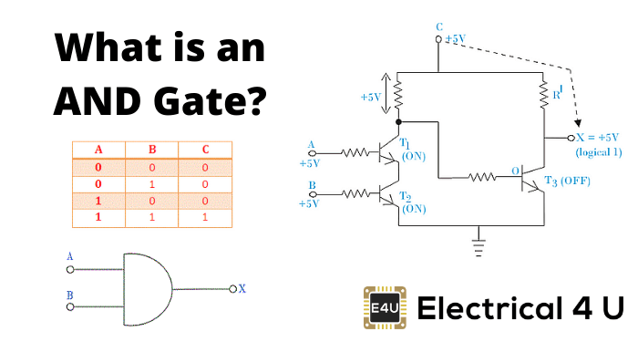
image source
Quantum computers also have gate and circuit concepts, but instead of logic gates processing 0 and 1, we represent quantum gates as matrices to operate on the state vectors of qubits.
Can any matrix be a quantum gate?
No! There is one important requirement: to become a quantum gate, a matrix \(U\) must be unitary, i.e. \( U^{\dagger} U = U U^{\dagger} = I \).
Why is unitary important?
- Invertible: quantum algorithms need this.
- Preserve length of their input: for any vector \(\ket{\psi}\), we have \( ||U\ket{\psi}|| = ||\ket{\psi}|| \). Actually, unitary matrices are the only matrics that can do this. Proof: see [1].
But why is length preservation important?
Because the amplitudes of each qubit must hold the normalization constraint, i.e. its length must always be 1, therefore using unitary matrices as quantum gates avoids violating this requirement.
The following sections introduce some common quantum gates, together with their circuit notations (we will talk more about circuits next week).
Single-qubit gates #
NOT gate (X) #
This gate is also called the Pauli-X gate, which is equivalent to rotating around the X-asis of the Bloch sphere by \(\pi\) radians.
\[ X = \begin{bmatrix} 0 & 1 \\ 1 & 0 \end{bmatrix} \]
\[ X^\dagger = X \ \ \ \ , \ \ \ \ XX = I \]
\[ XX\ket{\psi} = \ket{\psi} \]
\[ X( \alpha\ket{0} + \beta\ket{1} ) = \beta\ket{0} + \alpha\ket{1} \]
\[ X\ket{0} = \ket{1} \ \ \ \ , \ \ \ \ X\ket{1} = \ket{0} \]
\[ X\ket{+} = \ket{+} \ \ \ \ , \ \ \ \ X\ket{-} = -\ket{-} \]
\[ X\ket{i} = i\ket{i} \ \ \ \ , \ \ \ \ X\ket{-i} = -i\ket{i} \]
This gate is equivalent to rotating around the Y-asis of the Bloch sphere by \(\pi\) radians.
\[ Y = \begin{bmatrix} 0 & -i \\ i & 0 \end{bmatrix} \]
\[ Y^\dagger = Y \ \ \ \ , \ \ \ \ YY = I \]
\[ YY\ket{\psi} = \ket{\psi} \]
\[ Y( \alpha\ket{0} + \beta\ket{1} ) = -i\beta\ket{0} + i\alpha\ket{1} \]
\[ Y\ket{0} = i\ket{1} \ \ \ \ , \ \ \ \ Y\ket{1} = -i\ket{0} \]
\[ Y\ket{+} = -i\ket{-} \ \ \ \ , \ \ \ \ Y\ket{-} = i\ket{+} \]
\[ Y\ket{i} = \ket{i} \ \ \ \ , \ \ \ \ Y\ket{-i} = -\ket{-i} \]
This gate is equivalent to rotating around the Z-asis of the Bloch sphere by \(\pi\) radians.
\[ Z = \begin{bmatrix} 1 & 0 \\ 0 & -1 \end{bmatrix} \]
\[ Z^\dagger = Z \ \ \ \ , \ \ \ \ ZZ = I \]
\[ ZZ\ket{\psi} = \ket{\psi} \]
\[ Z( \alpha\ket{0} + \beta\ket{1} ) = \alpha\ket{0} - \beta\ket{1} \]
\[ Z\ket{0} = \ket{0} \ \ \ \ , \ \ \ \ Z\ket{1} = -\ket{1} \]
\[ Z\ket{+} = \ket{-} \ \ \ \ , \ \ \ \ Z\ket{-} = \ket{+} \]
\[ Z\ket{i} = \ket{-i} \ \ \ \ , \ \ \ \ Z\ket{-i} = \ket{i} \]
Hadamard gate (H) #
\[ H = \frac{1}{\sqrt{2}} \begin{bmatrix} 1 & 1 \\ 1 & -1 \end{bmatrix} \]
\[ H^\dagger = H \ \ \ \ , \ \ \ \ HH = I \]
\[ HH\ket{\psi} = \ket{\psi} \]
\[ H( \alpha\ket{0} + \beta\ket{1} ) = \frac{\alpha+\beta}{\sqrt{2}} \ket{0} + \frac{\alpha-\beta}{\sqrt{2}} \ket{1} \]
\[ H\ket{0} = \frac{\ket{0}+\ket{1}}{\sqrt{2}} = \ket{+} \ \ \ \ , \ \ \ \ H\ket{+} = \ket{0} \]
\[ H\ket{1} = \frac{\ket{0}-\ket{1}}{\sqrt{2}} = \ket{-} \ \ \ \ , \ \ \ \ H\ket{-} = \ket{1} \]
\[ H\ket{i} = e^{\frac{i\pi}{4}}\ket{-i} \ \ \ \ , \ \ \ \ H\ket{-i} = e^{\frac{-i\pi}{4}}\ket{i} \]
We can use H to put \( \ket{0} \) or \( \ket{1} \) into a superposition, or to distinguish between states such as \( \ket{+} \) and \( \ket{-} \).
Phase Shift gates #
These gates apply a phase shift to \( \ket{1} \) without changing \( \ket{0} \).
S gate #
\[ S = \begin{bmatrix} 1 & 0 \\ 0 & i \end{bmatrix} \]
\[ S( \alpha\ket{0} + \beta\ket{1} ) = \alpha\ket{0} + i\beta\ket{1} \]
\[ S\ket{0} = \ket{0} \ \ \ \ , \ \ \ \ S\ket{1} = i\ket{1} \]
\[ S\ket{+} = \ket{i} \ \ \ \ , \ \ \ \ S\ket{-} = \ket{-i} \]
\[ S\ket{i} = \ket{-} \ \ \ \ , \ \ \ \ S\ket{-i} = \ket{+} \]
\[ S^2 = Z \]
T gate #
\[ T = \begin{bmatrix} 1 & 0 \\ 0 & i \end{bmatrix} \]
\[ T( \alpha\ket{0} + \beta\ket{1} ) = \alpha\ket{0} + e^{\frac{i\pi}{4}}\beta\ket{1} \]
\[ T\ket{0} = \ket{0} \ \ \ \ , \ \ \ \ T\ket{1} = e^{\frac{i\pi}{4}}\ket{1} \]
\[ T^2 = S \]
Rotation gates #
More details in [1] and [4].
Rx gate #
\[ R_x(\theta) = \begin{bmatrix} cos{\frac{\theta}{2}} & -isin{\frac{\theta}{2}} \\ -isin{\frac{\theta}{2}} & cos{\frac{\theta}{2}} \end{bmatrix} \]
\[ R_x(\theta)( \alpha\ket{0} + \beta\ket{1} ) = (\alpha cos{\frac{\theta}{2}} - \beta isin{\frac{\theta}{2}} ) \ket{0} + (\beta cos{\frac{\theta}{2}} - \alpha isin{\frac{\theta}{2}} ) \ket{1} \]
\[ R_x(\theta)\ket{0} = cos{\frac{\theta}{2}} \ket{0} - isin{\frac{\theta}{2}} \ket{1} \]
\[ R_x(\theta)\ket{1} = cos{\frac{\theta}{2}} \ket{1} - isin{\frac{\theta}{2}} \ket{0} \]
\[ X = i R_x(\pi) \]
Ry gate #
\[ R_y(\theta) = \begin{bmatrix} cos{\frac{\theta}{2}} & -sin{\frac{\theta}{2}} \\ sin{\frac{\theta}{2}} & cos{\frac{\theta}{2}} \end{bmatrix} \]
\[ R_y(\theta)( \alpha\ket{0} + \beta\ket{1} ) = (\alpha cos{\frac{\theta}{2}} - \beta sin{\frac{\theta}{2}} ) \ket{0} + (\beta cos{\frac{\theta}{2}} + \alpha sin{\frac{\theta}{2}} ) \ket{1} \]
\[ R_y(\theta)\ket{0} = cos{\frac{\theta}{2}} \ket{0} + sin{\frac{\theta}{2}} \ket{1} \]
\[ R_y(\theta)\ket{1} = cos{\frac{\theta}{2}} \ket{1} - sin{\frac{\theta}{2}} \ket{0} \]
\[ Y = i R_y(\pi) \]
Rz gate #
\[ R_z(\theta) = \begin{bmatrix} e^{\frac{-i\theta}{2}} & 0 \\ 0 & e^{\frac{i\theta}{2}} \end{bmatrix} \]
\[ R_z(\theta)( \alpha\ket{0} + \beta\ket{1} ) = \alpha e^{\frac{-i\theta}{2}} \ket{0} + \beta e^{\frac{i\theta}{2}} \ket{1} \]
\[ R_z(\theta)\ket{0} = e^{\frac{-i\theta}{2}} \ket{0} \]
\[ R_z(\theta)\ket{1} = e^{\frac{i\theta}{2}} \ket{1} \]
\[ Z = i R_z(\pi) \]
R1 gate #
\[ R_z(\theta) = \begin{bmatrix} 1 & 0 \\ 0 & e^{i\theta} \end{bmatrix} \]
\[ R_z(\theta)( \alpha\ket{0} + \beta\ket{1} ) = \alpha \ket{0} + \beta e^{i\theta} \ket{1} \]
\[ R_z(\theta)\ket{0} = \ket{0} \]
\[ R_z(\theta)\ket{1} = e^{i\theta} \ket{1} \]
\[ R_1(\theta) = e^{\frac{i\theta}{2}} R_z(\theta) \]
\[ T = R_1(\frac{\pi}{4}) \]
\[ S = R_1(\frac{\pi}{2}) \]
\[ Z = R_1(\pi) \]
Multi-qubit gates #
C-NOT #
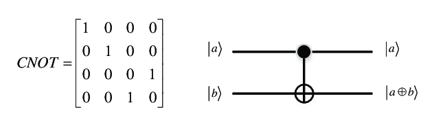
image source
- \( \ket{a} \) is the control bit.
- \( \ket{b} \) is the target bit.
- If the control bit is \( \ket{1} \) then flip the target bit. Otherwise do nothing.
Note that the above description only correct in the computational basis \( (\ket{0}, \ket{1}) \). In the \( (\ket{+}, \ket{-}) \) basis, for example, it might flip the control bit instead. See https://quantum.country/qcvc#the-controlled-not-gate for more details.
Programming #
https://colab.research.google.com/drive/1K5Vpzhk8H_zGjLY46sSQ7jrxeotSWrJ_?usp=sharing .
Summary #
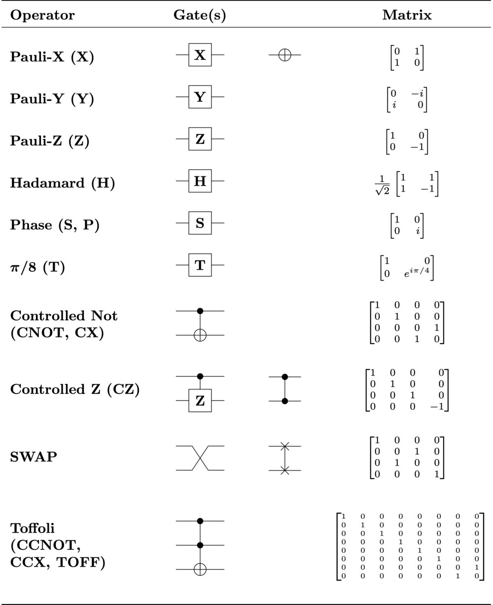
image source: [4].
Further readings #
- The Bloch Sphere - Ian Glendinning
References #
1. Part II: Introducing quantum logic gates - quantum.country - Andy Matuschak and Michael Nielsen.
2. Single-Qubit Gates - microsoft/QuantumKatas
3. Multi-Qubit Gates - microsoft/QuantumKatas
4. Quantum logic gate - Wikipedia
Since you've made it this far, sharing this article on your favorite social media network would be highly appreciated!
For feedback, ping me on Twitter.
All the information on this blog are my own opinions and do NOT represent the views or opinions of any of my past or current employers.
Published